
GNSS Test Engineering · Trajectory Inputs
GNSS Trajectory Import: Coordinate Frames, Time Scales and Motion Consistency
GNSS trajectory import turns a recorded or modeled path into motion that a simulator can reproduce. A file can parse successfully while placing the antenna at the wrong height, shifting the route in time or creating acceleration spikes between samples.
For receiver-test and HIL engineers, the first task is to define what every value means: the physical reference point, coordinate frame, units, state epoch and interpolation rule. Then verify the converted motion before judging receiver performance.
What makes an import usable? A versioned input file, an explicit interpretation contract and evidence that the simulator applies the intended state at the intended epoch. The example below is a project-defined exchange format for review, not a native NSG8000 file specification.
Use GNSS scenario design to plan events and acceptance objectives. This guide focuses on the data interpretation and checks needed to execute that plan. For the wider learning path, return to GNSS Simulation 101.
1. Agree the trajectory input contract
A column labeled altitude does not define a height reference. A timestamp does not establish its time scale. Keep these definitions in a versioned interface document or accompanying metadata, including fields that the file itself cannot express.
| Item | Required definition | Check before execution |
|---|---|---|
| File and parser | Format/version, encoding, delimiter, header rows, field order, numeric precision and missing-value rules. | Decode known rows; retain source file hash, parser version and conversion settings. |
| Reference point | Antenna reference point, IMU center or vehicle/model origin; any offset and who applies it. | Confirm position and velocity describe the same point. Apply each lever arm once. |
| Position and height | LLA, ECEF or a defined local frame; datum/reference-frame realization and coordinate epoch where relevant; units and vertical reference. | Check a known location and signed axis displacements. Record local origin and geoid model if used. |
| Time | Time scale, full epoch, units, state-validity instant, scenario-start mapping and rollover rules. | Reconstruct a unique absolute epoch for each state; distinguish it from file or packet arrival time. |
| Motion fields | Velocity and acceleration frames, units and derivative meaning; attitude convention if required; which fields are consumed, derived or ignored. | Compare redundant fields against the same motion model and reference point. Define which source is authoritative or reject conflicting fields. |
| Interpolation | Interpolation frame, method, derivative handling, sample cadence and allowable gaps. | Inspect motion between rows, including turns and segment boundaries. |
| Exceptions and lifecycle | Invalid rows, duplicates, out-of-order states, gaps, start/pre-roll, end-of-file, looping and live-input loss. | Specify reject, stop, hold or bounded extrapolation behavior and how exceptions are logged. |
Scroll horizontally to view all columns. Required fields and handling rules depend on the selected simulator configuration and interface.
2. Resolve LLA, ECEF, ENU/NED and height
LLA needs a datum and an unambiguous height
State whether latitude is geodetic, whether angles are degrees or radians, and how longitude is signed or wrapped. LLA-to-ECEF conversion uses the selected ellipsoid and ellipsoidal height, h.[1] Preserve enough precision for the position and dynamics tolerances of the test.
When the source supplies orthometric/MSL height H, use a compatible geoid separation Ng with the stated sign convention:
Illustrative conversion: H = 100 m and Ng = −30 m give h = 70 m.
The numbers above are hypothetical. Record the actual vertical datum and geoid model; an undocumented “MSL” value is insufficient for a precise conversion. Do not add geoid separation to a height that is already ellipsoidal.
A local frame needs an origin and axes
For a fixed-origin ENU frame, first obtain the origin position r0 in ECEF. Rotate the local displacement using the east, north and up basis vectors evaluated at that origin:[2]
ê = (−sin λ0, cos λ0, 0)
n̂ = (−sin φ0 cos λ0, −sin φ0 sin λ0, cos φ0)
û = (cos φ0 cos λ0, cos φ0 sin λ0, sin φ0)
Here φ0 and λ0 are the origin’s geodetic latitude and longitude. For the same origin and local basis, convert NED to ENU as (E, N, U) = (ENED, NNED, −DNED). Axis order and the vertical sign both matter.
For a fixed local basis, velocity and coordinate acceleration rotate with the same basis without a position translation. A moving local-level frame needs its own derivative treatment. ECI data also requires an epoch-dependent transformation; relabeling inertial coordinates as ECEF is invalid.
Check the physical point and attitude convention
A rotating body gives an offset antenna a different position and velocity from the model origin. Confirm lever-arm direction, units and frame, plus whether the source or simulator applies it. For attitude, define the body axes, reference frame, rotation direction and Euler sequence or quaternion ordering.
Vehicle conventions differ. NovAtel SPAN, for example, documents a vehicle frame with forward along +Y, right along +X and up along +Z.[8] Copying values into an interface that expects forward-right-down axes requires an explicit transformation. See the GNSS/IMU positioning guide for the broader fusion context.
3. Map state epochs to scenario time
Use the time when the motion state is valid. File read time, host receipt time and simulator application time are separate observations.
- Name the time scale. “GNSS time” is too broad. GPS Time is continuous without UTC leap seconds; other GNSS systems have their own references.[3] Use conversion data appropriate to the actual date rather than a permanently hard-coded offset.
- Retain a full epoch. UTC time-of-day needs a date. GPS seconds-of-week needs an unambiguous full week number. Resolve any truncated-week ambiguity from trusted context.
- Define the start mapping. State whether the file preserves its original epoch or is deliberately re-anchored to a new scenario epoch. Record that transformation; do not shift timestamps silently.
- Define boundary behavior. Test UTC midnight, GPS week rollover and leap-second handling where applicable. A POSIX timestamp and a leap-second-aware UTC representation require an explicit conversion policy.
T = 604800w + s; 0 ≤ s < 604800
Compare successive T values after resolving the week number.
A transition from (w, 604799.5) to (w + 1, 0.5) is one second forward. Subtracting seconds-of-week alone would produce a false backward jump. Store time with sufficient precision; integer week plus integer subsecond ticks can avoid losing fine resolution in a large floating-point epoch.
For live HIL input, also agree scheduling deadlines and the handling of late, missing or reordered states. A higher packet rate does not establish a more accurate trajectory or lower input-to-RF latency. The GNSS HIL testing solution defines the integration and measurement boundaries.
4. Treat NMEA as a source profile, not a complete motion contract
Identify the producer, firmware, sentence set, output configuration and validity rules. The following mappings use published NovAtel OEM7 log definitions; they illustrate source interpretation, not the accepted sentence set of an NSG8000 importer.
| Source sentence | Documented information | Import preparation |
|---|---|---|
| GGA[4] | UTC time-of-day, latitude/longitude in degrees and minutes, fix quality, MSL antenna altitude and geoid undulation. | Supply the date; decode hemisphere and units; verify the selected datum, time validity, fix policy and height conversion. |
| ZDA[5] | UTC time plus day, month and year. | Associate date/time with the correct position epoch. Check UTC validity and midnight transitions. |
| VTG[6] | True/magnetic track and ground speed in knots and km/h; no timestamp field in this documented sentence. | Require a verified epoch-association rule. Ground track is not body heading, and horizontal speed does not supply vertical velocity. |
Scroll horizontally to view the full mapping. The parser must handle the actual talker IDs and sentence variants in the supplied source.
For example, a latitude field 5109.0262,N means 51 + 9.0262/60 = 51.150436667°, rounded here to nine decimal places. Reading it as 51.090262° puts the route elsewhere. Validate checksums, missing fields and the source’s quality/status indicators before retaining a row.
Do not assume adjacent sentences belong to one epoch. Preserve source order and capture timing, then use the producer’s documented grouping behavior or another validated association rule. Keep rejected rows and reasons in the import report; never convert a missing coordinate or velocity into a silent zero.
5. Worked example: position, velocity and interpolation must agree
Illustrative input and expected calculations only; no measured product results are shown. This small synthetic trajectory checks coordinate conversion, epoch mapping and interpolation. Its one-second spacing is for arithmetic clarity, not a recommended operating rate.
Define the accompanying metadata
- Origin: WGS 84 ellipsoid, geodetic latitude 0°, longitude 0°, ellipsoidal height 100 m; fixed ENU axes at this origin.
- Point: one modeled antenna point. All rows describe that same point; no additional lever arm is applied.
- Epoch: full GPS week 2400, seconds-of-week 100000.000 at elapsed time t = 0. Scenario time is mapped to this epoch.
- Motion: E(t) = t² m, N(t) = U(t) = 0; vE(t) = 2t m/s; aE(t) = 2 m/s², for 0 ≤ t ≤ 2 s.
- Interpretation: position, velocity and acceleration are derivatives in the fixed ENU frame. Attitude is outside this point-motion example.
- Execution: use the stated analytic motion or a confirmed interpolation that reproduces it. Pre-roll is a separate segment; end at t = 2 s with the agreed stop procedure. No implicit loop, hold or extrapolation. This excerpt is not a complete smooth start/stop profile.
gps_week,gps_sow,e_m,n_m,u_m,ve_mps,vn_mps,vu_mps,ae_mps2,an_mps2,au_mps2
2400,100000.000,0.000,0.000,0.000,0.000,0.000,0.000,2.000,0.000,0.000
2400,100001.000,1.000,0.000,0.000,2.000,0.000,0.000,2.000,0.000,0.000
2400,100002.000,4.000,0.000,0.000,4.000,0.000,0.000,2.000,0.000,0.000
Project-defined normalized CSV for explanation. Map it to an approved import format before use; these headers and derivative fields are not a claim of native product compatibility.
Check the expected ECEF mapping
The WGS 84 semi-major axis is 6378137 m. At this origin, r0 = (6378237, 0, 0) m, with east along ECEF +Y, north along +Z and up along +X. Therefore:
vECEF(t) = (0, 2t, 0) m/s
aECEF(t) = (0, 2, 0) m/s²
At t = 2 s, the expected ECEF position is (6378237, 4, 0) m. Here U = 0 describes a fixed tangent plane, not an exactly constant ellipsoidal height along an extended route.
Check the motion between rows
Across each one-second interval, the position difference equals the average endpoint velocity multiplied by the interval: 1 m = (0 + 2)/2 × 1 s and 3 m = (2 + 4)/2 × 1 s. This equality is exact for this constant-acceleration example; it is not a universal identity for arbitrary motion.
At t = 0.5 s, the intended motion has E = 0.25 m and vE = 1 m/s. Linear position interpolation from E = 0 to E = 1 instead gives E = 0.5 m, with a constant segment slope of 1 m/s. It misses the intended midpoint position by 0.25 m and cannot reproduce the changing velocity throughout the interval.
A matched position-and-velocity interpolation, such as cubic Hermite interpolation with these endpoint derivatives, reproduces this polynomial segment. Confirm what the actual importer uses and whether it honors derivative fields. Smoothing or independently interpolating position, velocity and acceleration can produce a different motion model.
Check starts, stops, turns and file joins as well as midpoints. Handle longitude and attitude-angle wrapping explicitly; quaternion interpolation also needs a declared rotation convention. Retiming this two-second motion to one second would double velocity and multiply acceleration by four; changing row timestamps without updating the motion fields would make the input inconsistent.
6. Run preflight checks, then verify execution
- Decode and account for the source. Check field count, finite values, ranges, status, precision and units. Report total, accepted and rejected rows, with reasons and affected epochs.
- Normalize coordinates and time. Verify a known static point, signed axis movements, height reference and full epochs. Use independently checked test vectors; a round-trip through one converter alone can preserve a shared error.
- Check continuity and dynamics. Inspect sample intervals, gaps, duplicates and ordering. Evaluate the interpolation on a finer diagnostic grid and at boundaries; compare its derivatives with any supplied motion fields. Choose tolerances from the test needs and numerical precision.
- Verify the simulator interpretation. Retain decoded previews, applied-state logs or other agreed simulator-side evidence at selected epochs, including between source rows. Check start mapping, end behavior and exception handling. A successful parser report establishes only part of this evidence.
- Verify RF and receiver behavior separately. Use the agreed RF observation method where RF-state or timing acceptance is required. Align receiver PVT with truth at its measurement epoch; document receiver validity and errors without treating its estimates as an exact echo of imported truth.
For recorded positions, “truth” here means the approved test reference. Importing a noisy receiver track does not establish that it was the vehicle’s true path. Preserve raw data and document any cleaning, smoothing or resampling.
| Observed symptom | Possible input cause | Discriminating check |
|---|---|---|
| Large vertical offset | MSL/ellipsoid mismatch, wrong geoid sign or duplicated correction. | Trace one original height through each conversion and compare its declared reference. |
| Mirrored or rotated route | ENU/NED swap, hemisphere sign, wrong origin or axis convention. | Import separate known east, north and up displacements. |
| Route shifted in time | UTC/GPS confusion, missing date, wrong week or unintended re-anchoring. | Verify a known absolute epoch and a marked motion event on the agreed time base. |
| Velocity or acceleration spikes | Position quantization, repeated/backward epochs, gaps, join discontinuities or interpolation behavior. | Inspect raw rows and reconstructed derivatives around the affected interval. |
| Mismatch grows with rotation | Wrong antenna reference point, lever arm or attitude convention. | Compare model-origin and antenna-point states with the same rotation definition. |
These are diagnostic hypotheses, not automatic fault classifications. Scroll horizontally to view all columns.
Record a verified mismatch as a failure. If applied-state or RF evidence needed by the agreed check is unavailable, record that item as not verified. Keep the source, converted file, hashes, parser/configuration versions, epoch/frame definitions, exception report and execution evidence together. Use the receiver validation test plan to connect this evidence to overall acceptance.
Coordinate acceleration is not an IMU sample. The second derivative of trajectory position is not automatically accelerometer specific force. Sensor generation requires agreed gravity, rotating-frame, body-axis, angular-rate and sampling conventions. GNSS RF representing a moving antenna does not physically move a stationary IMU.
7. Confirm trajectory import compatibility for the selected bench
The NSG8000 product page lists trajectory import including NMEA and custom formats. The HIL solution defines motion fields, conversions and timing behavior through a project interface review. File import and live motion injection need their own agreed mappings.
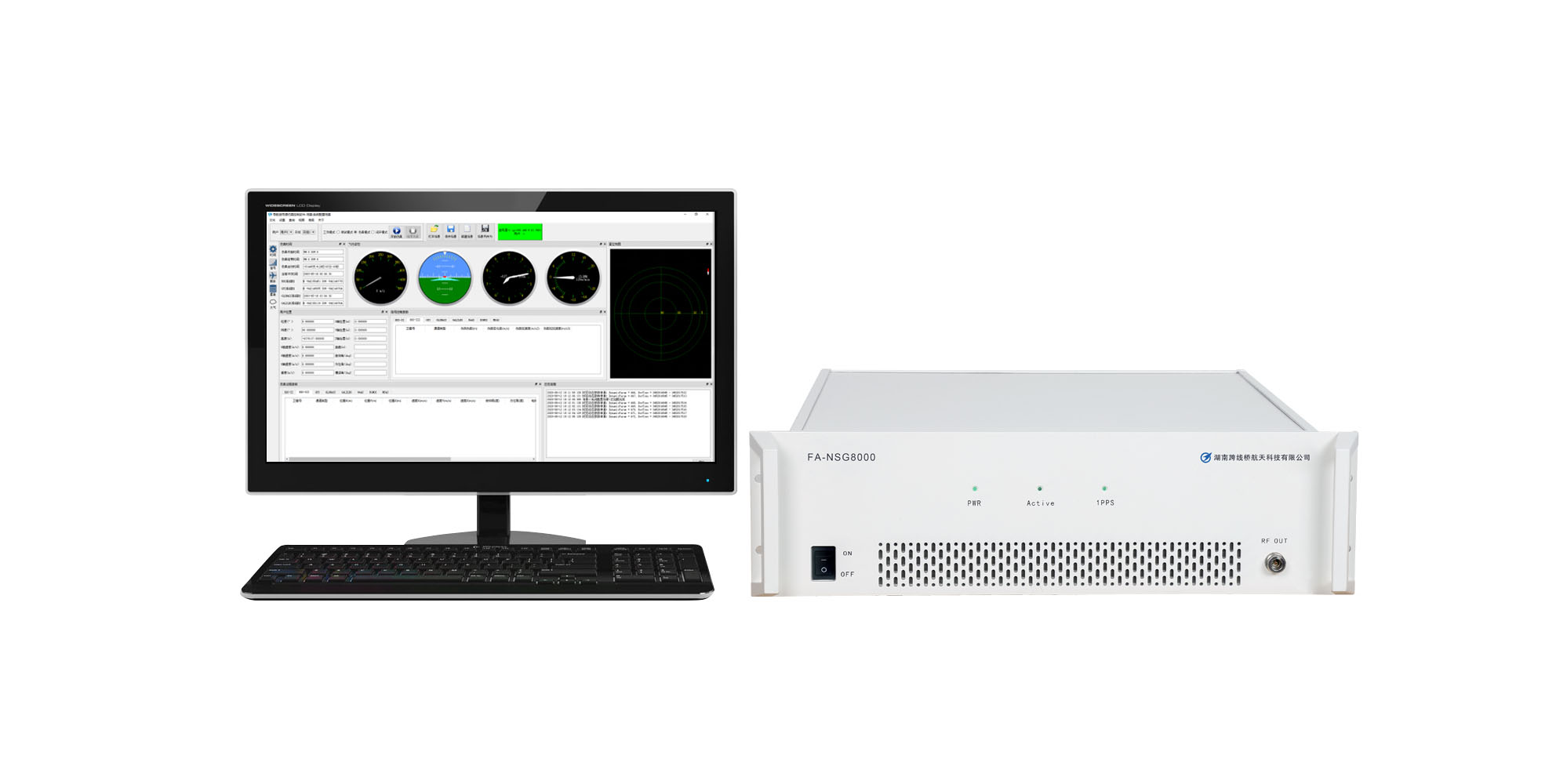
NSG8000 trajectory and HIL configuration
Review the source format, required GNSS signals, motion fields and timing objectives against the selected hardware, software and interface configuration.
View NSG8000 and configuration details →Confirm the accepted sentence set or file schema, units, coordinate/height interpretation, timestamp mapping, interpolation and gap/end behavior before running customer data. Agree any adapter work and the evidence available for checking applied states. General CSV support elsewhere in the industry does not establish compatibility with this configuration.
For example, Safran’s Skydel documentation explicitly exposes CSV column/unit mapping and interpolation choices, and warns about position precision and ECI epoch dependence.[7] This illustrates why importer-specific documentation matters; its controls and formats are not NSG8000 specifications.
GNSS trajectory import FAQ
Can a GGA-only file define the complete trajectory?
GGA can provide position and UTC time-of-day, but it does not provide a calendar date, full velocity vector or attitude. Supply the missing definitions and confirm how the selected importer reconstructs motion between positions.
Can I convert NED to ENU by swapping north and east?
Also reverse the vertical sign: ENU = (E, N, −D) for the same origin and basis. Confirm whether the frame is fixed at one origin or moves with the platform.
Does resampling a 1 Hz file to 100 Hz add motion fidelity?
It adds samples of an interpolation model, not new source observations. Fidelity depends on source precision, dynamics and the interpolation assumptions. Validate the reconstructed motion against the intended reference.
Should track over ground be imported as vehicle heading?
Only if the test explicitly justifies that relationship. Reversing, sideslip and near-zero speed can separate track from body orientation. Use an independently defined attitude source when the test needs body heading.
Is a correct trajectory preview enough to validate GNSS RF timing?
No. A preview checks interpretation at the displayed points. RF-state timing requires the agreed observation boundary, a common time base and supporting RF evidence. Receiver estimates add their own processing and measurement behavior.
Review your trajectory format and test interface
Start with your source software/file type, receiver model, required GNSS signals and intended motion. Add coordinate and height references, time scale, sample cadence and whether the test uses file playback or live HIL input.
Request a technical review to define the field mapping, any conversion work, configuration requirements and acceptance checks. A short non-confidential sample and interface documentation can follow during that review.
Technical references
Source-specific examples support interpretation checks; they do not imply cross-product file compatibility.
- ESA Navipedia: Ellipsoidal and Cartesian Coordinates Conversion.
- ESA Navipedia: Transformations between ECEF and ENU coordinates.
- ESA Navipedia: Time References in GNSS.
- NovAtel OEM7: GPGGA.
- NovAtel OEM7: GPZDA.
- NovAtel OEM7: GPVTG.
- Safran Skydel User Manual: Settings—Vehicle.
- NovAtel OEM7: Definition of reference frames within SPAN.